How We Render Extremely Large Point Clouds

In this article, we explore state-of-the-art point cloud rendering techniques and show how we built our custom compute-based render pipeline.

We were tasked with rendering very large point cloud data sets, measured in the order of millions of points. Not only did this have to run at interactive frame rates, but it needed to look good in scenes at eye level. This meant we needed some form of point rejection to avoid rendering points that should be occluded. We achieved this by implementing state-of-the-art whitepapers and some Magnopus magic to get it all working in the Unity game engine.

The Problem

First of all, why do we need this tech? After all, there are a couple of point cloud plugins on the Unity Asset Store that render point clouds and one in particular that touts the ability to render datasets of billions of points. Unreal even has one built-in to the engine that’s free to use. The reason essentially boils down to the fact that these tools are generally meant for visualizing datasets without prioritizing visual quality. That’s not to say that any of these plugins do a bad job at rendering the point clouds; there are just some tradeoffs that these techniques leverage that we would rather not make.

The Status Quo

The simplest approach to rendering point clouds is leveraging the point rasterization pipeline present in many rendering APIs. On the surface, you may think that since the APIs have a first-class rendering mode for points, it would be the fastest way to render point data to the screen. However, once you delve into the APIs rasterization rules, you will find that under the hood, each point is essentially expanded into a two-triangle camera-facing quad.

The problem with this technique is that it produces very small triangles which are not optimal for modern GPU architectures. Every pixel rendered by a GPU evaluates at least four times in a 2x2 tile to compute derivatives that get used for things such as texture mipmap selection. This is something that cannot be disabled and you are paying for whether you use the derivatives or not. Depending on the specific GPU architecture, the minimum tile size may be much larger than that.

Some point cloud renderers opt to substitute a small mesh for each point in the point cloud to give volume and artistic style to the points in the cloud. This does give more control over the look, but generally exacerbates the issues mentioned above with very small triangles.

*The Magnopus office scan rendered with unlit pyramids in place of each point.*

For most cases, this is a nonissue due to the fact that the number of points is typically few enough that modern GPUs churn through the tiny triangles with ease. However, for the case of rendering extremely large point clouds, the performance issues are very noticeable.

Many point cloud renderers employ some form of level-of-detail (LOD) to reduce the number of points submitted to the GPU. The fewer points that are sent to the GPU, the faster it will be at rendering them. This also has the added benefit of reducing the amount of flickering and aliasing when the point clouds are far enough from the user. However, this usually results in holes in the point cloud at large distances despite there being plenty of data in the raw point cloud to populate all pixels in that area.

Another common technique is to take the point cloud data and transform it into another data structure so it can be rendered via some other technique. This can be running an algorithm that transforms a point cloud into a 3D mesh or voxels. There is also a lot of research in the space of 3D Gaussian splatting which is a form of point cloud rendering that can produce some very compelling images. Unfortunately, each of these techniques are lossy ways of rendering a point cloud. It’s something we are keeping an eye on, but not quite a fit for our current needs.

The Solution

The graphics pipeline is highly optimized for triangulated meshes, and as we have seen above, shoehorning point cloud rendering into that pipeline has resulted in some inefficiencies. The solution is to ignore the graphics pipeline completely.

Instead, we built an entirely new rasterization pipeline via the GPU’s compute shader pipeline. Compute shaders enable general-purpose computing on the GPU and as a result, there are no assumptions made about the data coming in and out of the pipeline avoiding the inefficiencies mentioned in the above techniques.

Four whitepapers are at the heart of our point cloud rendering technique:

Rendering Point Clouds with Compute Shaders and Vertex Order Optimization for efficiently writing the cloud data to the screen buffer.
Real-time Rendering of Massive Unstructured Raw Point Clouds using Screen-space Operators for point rejection and hole filling.
Real-Time Continuous Level of Detail Rendering of Point Clouds for a clever Level of Detail implementation.
Software Rasterization of 2 Billion Points in Real Time for improved data throughput.

First, let’s explore the relevant parts of each of these papers before we talk about how we pieced them together to make our custom point cloud rasterization pipeline.

Ordering and Rendering Points

The first, and most important part of the puzzle is rendering the raw point cloud data on screen. As mentioned before, we prefer to avoid the graphics pipeline. The whitepaper Rendering Point Clouds with Compute Shaders and Vertex Order Optimization spells out exactly what we want to do in its title. This paper has some clever tricks that we make use of to efficiently render point clouds to the screen as well as solve aliasing problems that come with the territory of very large point clouds.

Reordering Points for Big Performance Gains

Surprisingly, one of the biggest improvements to performance comes by simply reordering the points in the dataset. Since point clouds contain points with no connectivity information, we are free to reorder the points in the dataset. If you load a dataset in the order that a scanner has saved it out, you will usually see that neighboring points are physically far from one another. This is because the scanners typically capture a color+depth image and then write out the points in the order they are in the source image (i.e. left-to-right, top-to-bottom). Since each pixel can have a wildly different depth to them, discontinuities are unavoidable.

To solve this, the paper suggests sorting the points using Morton ordering and shuffling contiguous blocks of points around. Morton ordering is also known as Z-ordering. It’s a way of ordering three-dimensional points in a one-dimensional array so that each point in the array is adjacent to the next closest point in three-dimensional space. This ensures that when the GPU launches a wave of threads, the points within the wave are projected onto a small two-dimensional area on the screen which in turn reduces the chances of expensive cache misses.

The next step is to shuffle blocks of points within the dataset. This may sound counterintuitive at first since we just neatly organized our dataset. But the reason for the shuffling is that when the data is sorted perfectly, you increase the chance that two or more waves that are in flight at the same time map points that occupy the same screen pixel. Since only one thread can safely write to a memory address at the same time, the other threads will stall out waiting for their turn to write their data to the buffer. By shuffling the points in blocks at a minimum of a wave’s execution size, we retain order within the wave but decrease the chance that multiple waves are fighting over the same pixel.

Rendering the Points

Now that the points are in an optimal ordering, we need to write the points to the screen somehow. The paper leverages atomic shader instructions to efficiently render the scene. There are multiple techniques that the paper explores, but the one we are interested in is what they call “high-quality shading” which is not only fast but solves the issue of aliasing.

The technique requires creating two array buffers; one for depth information, and another for color data. Each element in these buffers map to a single pixel on-screen. The depth data is stored in 32-bit unsigned integers, and color data in two 64-bit unsigned integers. The color data stores red color in the upper 32 bits, and green in the lower 32 bits of the first integer. The second integer stores blue in the upper bits, and a counter for the number of color values summed in that pixel within the lower bits.

In the first pass, all points are projected onto the screen and the closest point’s depth value is stored in the buffer. Then, in the second pass, we re-project all the points, but this time store color data for each point that is within an epsilon of the recorded depth value. When a point is within the epsilon of the stored depth data, the color information is added to the color buffers and the point counter is incremented by one. This is all done with atomic add functions which are fast and avoid any race conditions when two or more points are projected to the same pixel at the same time. In a final pass, this data is then converted to color data and written to the framebuffer. The summed color data is divided by the number of points that were accumulated for each pixel giving the final color.

Point Rejection and Hole Filling

Once we have the points written to the screen, we need to fill any gaps between the points efficiently. Because the points are infinitesimally small and map to a single pixel, we will often see points of distant objects rendered between points that are far closer to the camera. Visually this is confusing. You would expect the object closer to the camera to occlude anything behind it, which is why we need to reject or remove any points that should be occluded before running the hole filling algorithm.

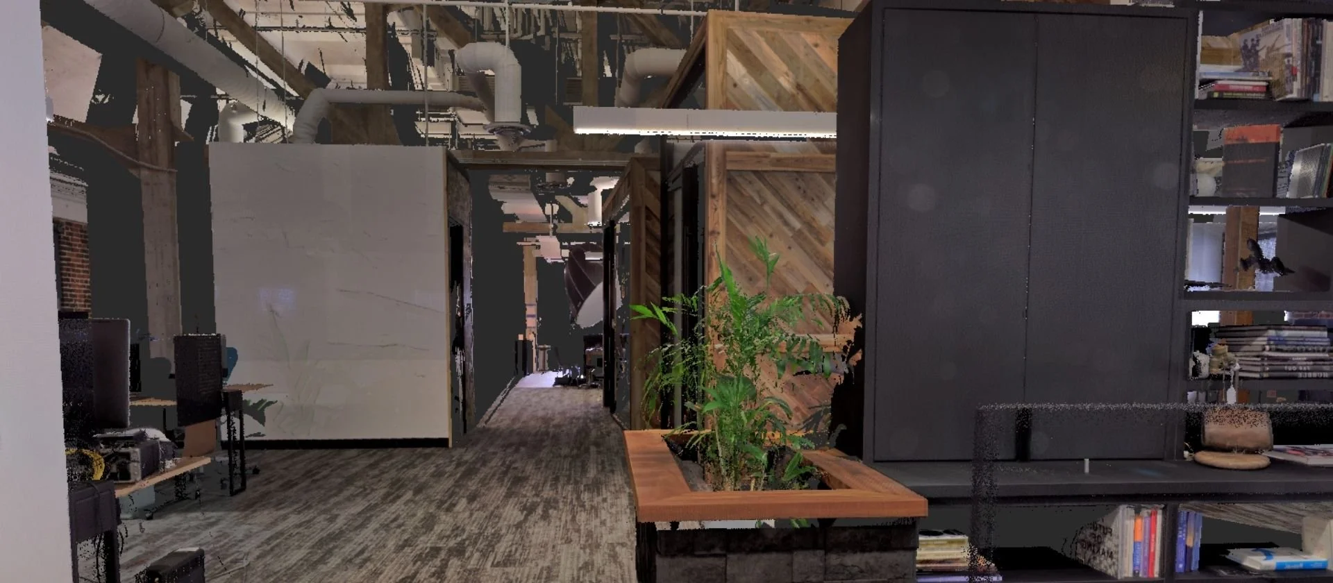
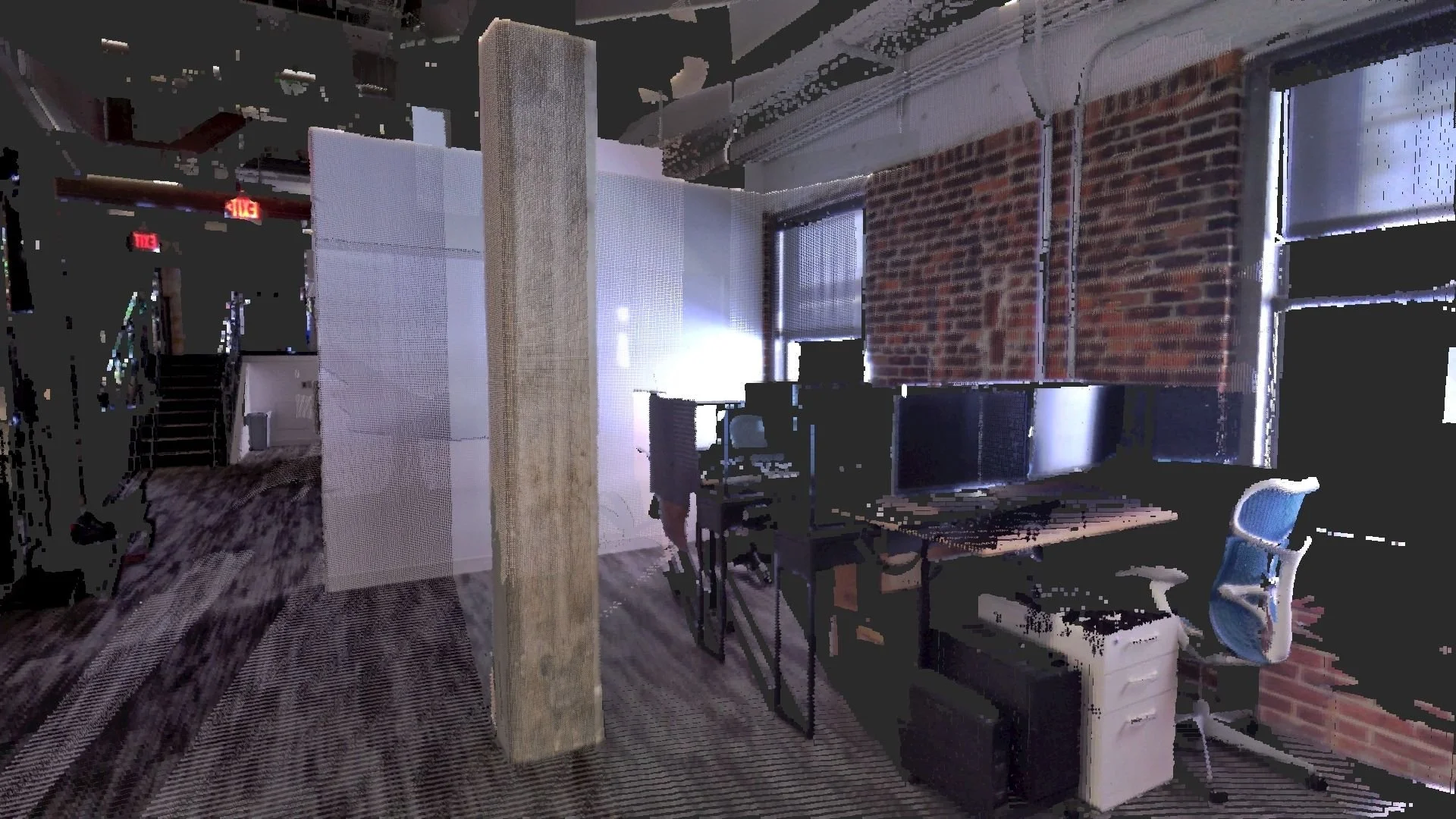
Take the following screenshot for example:

There is the top of a chair in the foreground, but we can see straight through it to the desks behind it which is not correct.

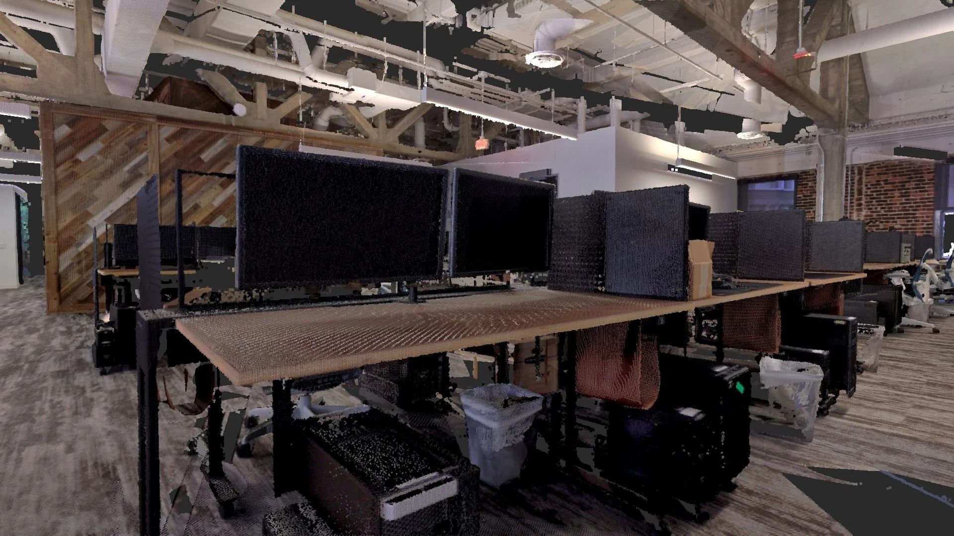
Now let’s take a look at what the scene looks like with point rejection enabled:

The top of the chair is much more visible in this shot and the desks behind are fully occluded. Unfortunately, this now creates a problem where we have a lot of empty space between the points.

The hole filling algorithm expands each of the points that remain until the empty space is filled in. Here is what the final render of the scene looks like:

The chair finally looks solid and occludes the scene behind it, just as we would expect to see.

The paper Real-time Rendering of Massive Unstructured Raw Point Clouds using Screen-space Operators details how to reject distant and occluded points, as well as fill the resulting holes.

To reject points, each point in the image is evaluated against other nearby points in a 7x7 grid where the evaluated pixel is directly in the center. For each point in the grid that is closer to the camera, a shader calculates the largest cone about the center that can exist without intersecting any of the other points. Then, if this cone is smaller than a defined threshold, the point is determined to be occluded and is removed from the buffer.

To fill the resulting holes, a recursive point expansion algorithm is run. With each iteration, every empty pixel that has neighboring pixels with color data updates its color to the average of those neighbors. The same is done with the depth information. The kernel is run three times to expand a point as far as the 7x7 bounds used in the rejection pass.

Level of Detail

When we deal with very dense point clouds, there will be times when many points project to a single point on screen. This becomes a large bottleneck, because our rendering logic uses atomic operations and many threads become blocked while they wait their turn to write data to the pixel. While the points will average together nicely with the antialiasing logic, we quickly get a diminishing return on our efforts, especially considering the performance cost. The solution here is to reduce the number of points in a way that doesn’t introduce more holes or negatively affect the frame.

Typically, other point cloud renderers use a tile-based LOD system. This would reduce the number of points so that data contention is not an issue, but because the density can only be reduced by the resolution of a tile, you will often get holes appearing in the cloud as well as visual pops.

The paper Real-Time Continuous Level of Detail Rendering of Point Clouds presents a new LOD system that is specific to point clouds which it calls Continuous Level of Detail, or CLOD for short.

Since point cloud points have no connectivity data, we can easily discard a point if we determine that it does not make any meaningful difference in the final frame. Therefore we can operate at the granularity of a single point for LOD generation which is exactly what the CLOD technique does. This eliminates visual pops as well as minimizing the number of holes created.

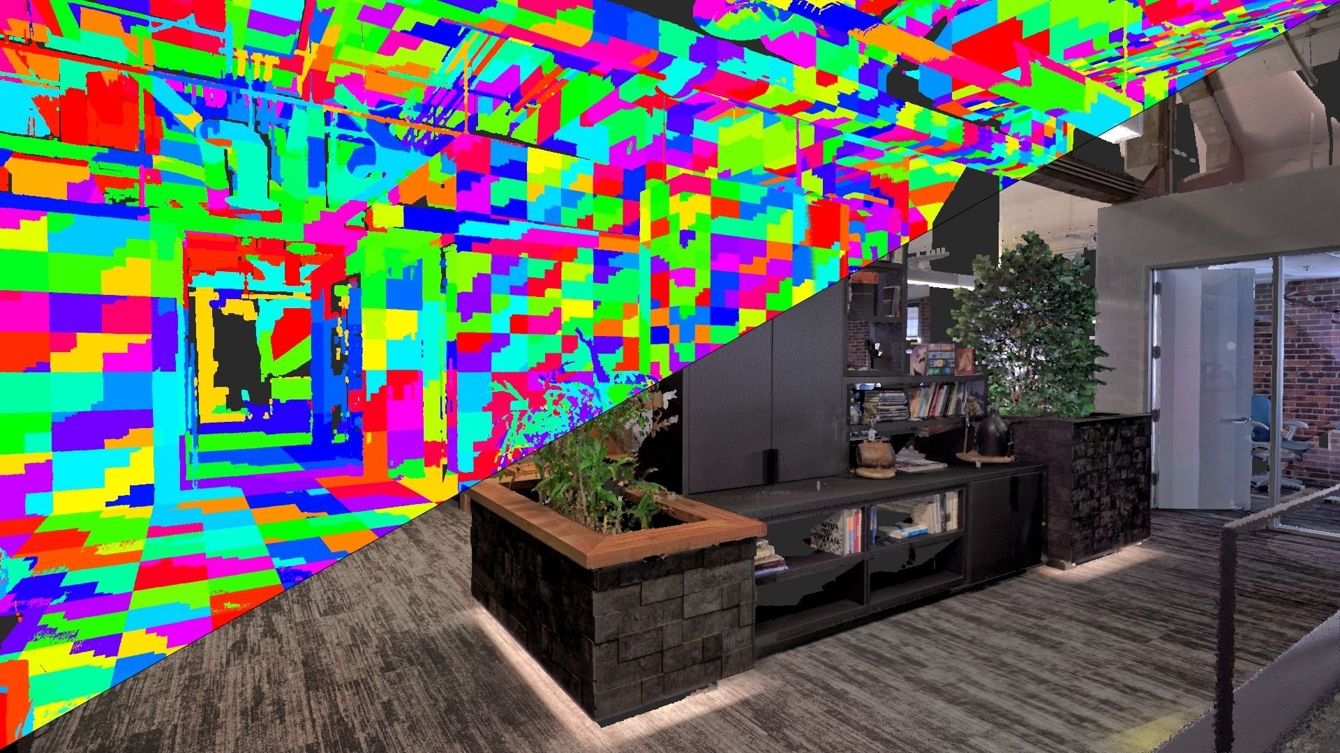
Each point in the cloud is assigned an LOD value of 0 through 3. The vast majority of points are usually categorized under level 3 which is the full detail cloud. Then, every 1 meter in each dimension, a single point is chosen to be categorized in LOD 0. The same is done for every 0.5 meter with LOD 1, and 0.25 meter for LOD 2. The points in LOD 0 through 2 are proxy points that are representative of the points that exist in their respective volumes. For instance, a point of LOD 0 represents all points in the 1x1x1 meter volume around it. We also average the color of all of the points in the respective volume so there are no color aliasing issues.

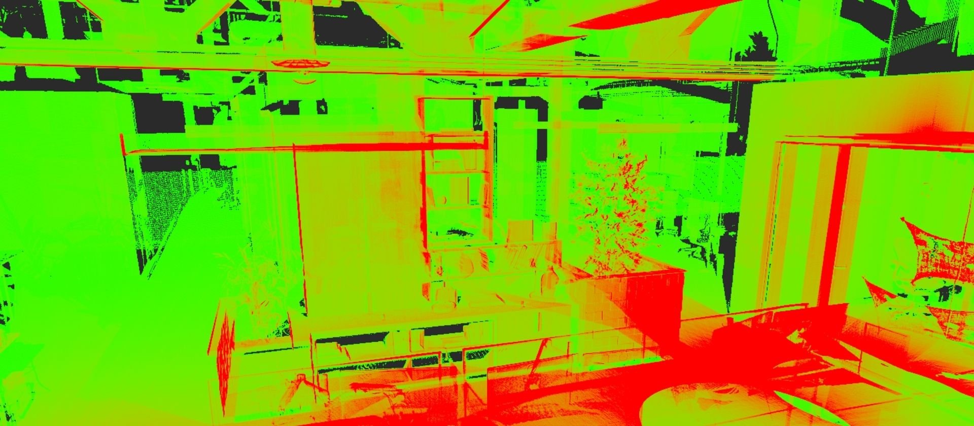
Both screenshots below are of the exact same view.The left view shows the full point cloud dataset with colors visualized, and the right view shows the LOD points that were selected. In this debug view, red is used for LOD 0, green for LOD 1, and Blue for LOD 2. LOD3 is not rendered since it is all of the other remaining points in the dataset. Notice that the LOD points are more uniformly distributed and the density varies between LOD levels as you would expect.

Then, at runtime, we iterate over all points in the cloud to evaluate if they should be visible, and copy the visible points into a new point cloud that is then rendered. A benefit is that we can amortize the cost of generating this reduced point cloud over multiple frames. This comes at the cost of empty space at the edges of the screen if the camera moves too quickly.

To evaluate if a point is visible, we first do a frustum check, and if it passes that, we test the point’s distance from the camera to the LOD level assigned to the point. Since our LOD levels are coarsely organized between four levels, we would see a harsh line in the point cloud where the distance threshold between LOD levels exists. To avoid this, we assign a randomized and normalized weight for each point to smoothly blend between each LOD. This works beautifully and when we combine that with our hole filling technique, it becomes a practically invisible transition.

Optimizing Memory Throughput

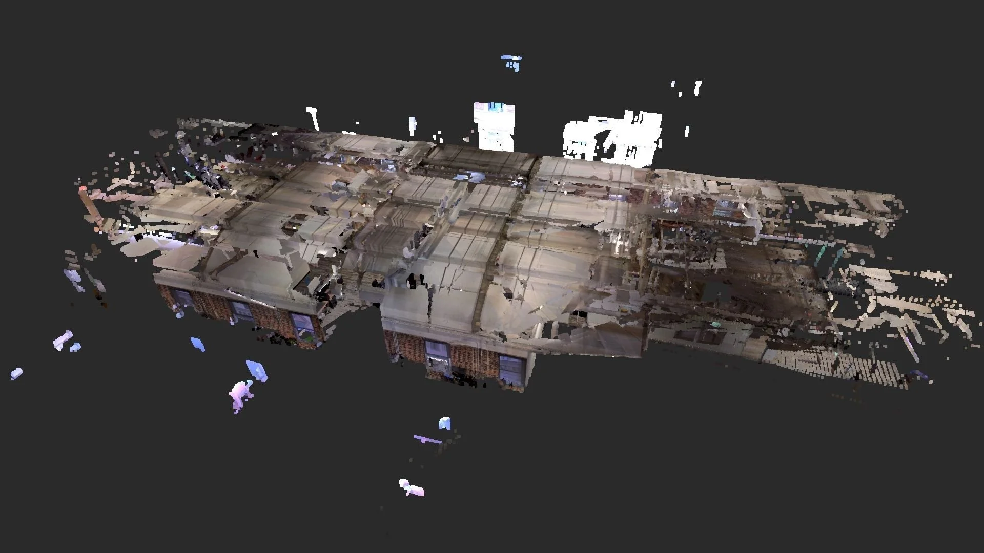
The Magnopus point cloud dataset with a batch visualization mode.

Our final paper, Software Rasterization of 2 Billion Points in Real Time, outlines how we can improve the GPU memory throughput.

It’s no secret that point clouds are memory intensive. We’re storing information for millions of points, and each point has position and color data associated with it. This can quickly balloon into multiples of gigabytes for a modestly sized point cloud if not addressed properly.

Fortunately for us, in recent years, memory has become plentiful and cheap, so storing this data isn’t as daunting as it may seem. However, while memory has increased, the speed at which it can be accessed (also known as data throughput) hasn’t kept up. This has become a large bottleneck in rendering performance.

The paper presents a method of organizing the points into blocks of equal size (10,240 points) and physical locality. A new buffer is created with the metadata of the axis-aligned bounding box for all of the points as well as what range of points in the point cloud it relates to. This enables two things; efficient culling of large blocks of points outside of the frustum, and informs us how much detail can be resolved in the area when projected onto the screen.

Knowing how large that block of points is on screen enables the next part of what makes this paper so great. We are now able to reduce the number of bytes that represent the positions of each point greatly reducing the amount of data passed around the GPU.

Traditionally we store point cloud location data with a floating point value for the x, y, and z coordinates. Floating point values give us the flexibility to place our points anywhere in the world we like with little thought to the backing data. However, since it is ultimately just binary data, you cannot represent any conceivable number since that would require an infinite number of bits. Floating point values are designed so that most of the precision exists around the value 1.0 and becomes less precise the closer the number is to zero or infinity. Furthermore, all bits in a floating point number need to be present to make sense of it.

Another way we can store the point cloud positional data is in fixed-point notation. That means that each increment we make in the binary value, the number increases by a fixed amount. For example, a binary value of 21 with a fixed point resolution of 0.25 would evaluate to the number 5.25. Additionally, we can split the binary representation up and still make some sense of what the number is which this paper takes advantage of.

Each point’s position is converted into fixed-point notation to a resolution of 30 bits. The position stored in these 30 bits expresses a normalized location between the bounds of the axis-aligned bounding box that contains the point. The fixed-point number is then broken into 3 segments of 10 bits. The segments are then reorganized so that the top 10 bits of the x, y, and z coordinates are packed into a 32 bit unsigned integer with two bytes of padding. The same is done for the middle and lower bits. Then three arrays are created that store the high, medium, and low precision data respectively. We will refer to this technique here on out as “quantized batches”.

Now, when we evaluate each block of points, we project the bounding box into clip space to know if we need 10, 20, or 30 bits to reconstruct the world position at the resolution of the screen the points map to. Here you can see a visualization of this where high precision points are colored red, medium green, and low blue.

Putting it All Together

Hopefully, by now you can see that we have all the components to make an efficient point cloud renderer. We can dynamically generate an LOD, project the points onto the screen while minimizing the data throughput, reject points that should be occluded, and fill resulting holes. However, before we do any of that, we need to import our data.

The Import Process

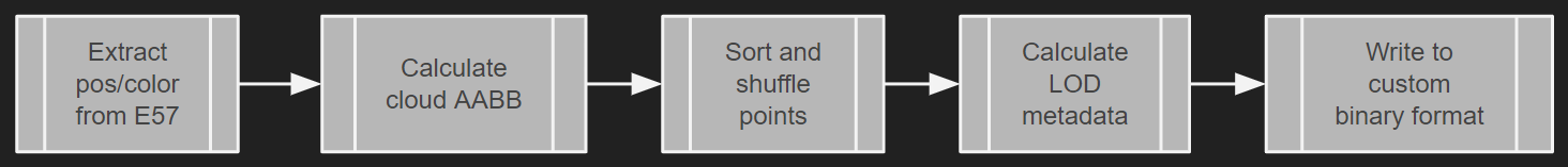
We wrote a custom Unity asset importer for E57 point cloud files. A native plugin is used to parse the E57 file to retrieve all position and color data and load it into memory. We then get the componentwise min and max coordinates and store that as our axis-aligned bounding box for the entire cloud.

All points are then sorted via Z-order and shuffled. The points are split into batches of 10,240 points which is the minimum batch size suggested in our last paper. Every other batch is swapped with a batch at the end of the scan data. For instance, the second batch is swapped with the second-to-last batch. We chose this approach because it sufficiently shuffles the data while doing so in constant time.

Next, we identify all of our LOD points and write that data into the alpha component of the color. Since our point cloud data contains no transparency data, we use that to store the LOD metadata. To determine which point is LOD 0, 1, or 2, we keep track of which point is closest to the center of each 1x1x1 meter cube, 0.5x0.5x0.5 meter cube, and 0.25x0.25x0.25 meter cube respectively and update the metadata accordingly.

Last, we write all of the data into a custom binary file format alongside some header data.

Configuration

*A view of our large point cloud rendering feature inspector in Unity.*

We first need to prepare our point cloud rendering system by pre-processing and uploading the point cloud data to the GPU as well as creating some necessary buffers for the rendering system to operate on. Because the problem of rendering large point clouds efficiently is still unsolved, we architected this system to be highly configurable and flexible. You can choose how point clouds are represented in memory, enable or disable the continuous level of detail system, and set the aggressiveness of the point rejection logic to name a few. The system will adapt to what is configured, which means the logic outlined below may look a bit different.

I’ve decided to focus on the most interesting configuration below – a novel merging of both the continuous level of detail system as well as the quantized batches.

System Preparation

When uploading point cloud data, we upload all of the point data in multiple buffers. The position data is stored in high, medium, and low precision uint structured buffers which store the segmented fixed-point position information. The fourth buffer is a structured buffer of uint containing color information. The red, green, and blue color data is each stored in a single byte and combined together into an unsigned integer. The remaining byte is used to store the LOD level. A fifth buffer is used to store batch information. Each entry in the batch buffer represents 10,240 points and stores information about the axis-aligned bounding box, and the offset into the point cloud where the batch starts. A batch size value is also stored. Since each batch size is a max of 10,240 points, you may think there is no need to store the size of the batch. However, this becomes useful later when we are dealing with the generated LOD point cloud.

HLSL
struct PointCloudBatch
{
	float3 Min;
	uint Offset;
	float3 Max;
	uint Count;
};

StructuredBuffer<PointCloudBatch> PointCloudBatches;
StructuredBuffer<uint> PointCloudColors;
StructuredBuffer<uint> PointCloudPositionsLow;
StructuredBuffer<uint> PointCloudPositionsMedium;
StructuredBuffer<uint> PointCloudPositionsHigh;

We then need to create some buffers for the algorithm to use. First, we create a set of buffers that represent the LOD point cloud that we actually render to the screen. This consists of the same five buffers mentioned above and the number of elements is defined by the user which is the upper-bound of how many points can be rendered at any time. If the user also opts to amortize the LOD generation over multiple frames, we duplicate these buffers so we can double-buffer the point clouds which comes at the cost of additional memory usage.

Lastly, we create a framebuffer attribute buffer. Each element in this buffer corresponds to a single pixel in the backbuffer and stores information about the rasterized cloud’s depth and color. This will later be copied to the framebuffer so it can be presented on screen. We need this as an intermediate buffer because a framebuffer cannot be directly used in a compute shader and we need the color data represented as uint values for the atomic operations we take advantage of in the shaders.

The Custom Point Rendering Pipeline

Now that we have the point clouds imported, uploaded, and intermediate buffers created, we can render it to the screen. Below is a visualization of our custom point cloud rasterization tech.

Our first step is to generate our LOD point cloud. A compute shader is executed that projects points into clip space and evaluates if they pass the CLOD system detailed above. Since we have our points grouped into batches, we can have each thread in the compute shader evaluate many points instead of a one-point-to-one-thread mapping. This allows us to first test the containing batch’s bounding box against the view frustum and exit the shader early if it’s not visible. This gives us a measurable improvement in the LOD generation pass that would not have been possible if we had not organized our points into batches. For the batches that are visible even slightly, we iterate over each point and only copy it when it passes the CLOD check. Before we copy the point over, we project it into world-space. This is necessary because the LOD cloud can contain points from multiple point clouds and world-space is common between them.

Since we have millions of points to iterate over and potentially copy, this can be an expensive part of the process. Because of that, there is an option to amortize the cost over multiple frames. When this is amortized, an upper-bound is set for the number of points to evaluate in a given frame, and we keep track of the last evaluated point so we can resume in the next frame. The LOD point cloud is double-buffered so we don’t see partial culling results. Once all points have been evaluated, we swap the buffers so that the old buffer is now being written to, and the new buffer is now being presented.

Next, we render the LOD point cloud to our attribute buffer. Here is the struct we use for this buffer.

HLSL
struct PointCloudPixelAttributes
{
    uint colorCount;
    uint3 color;
    uint depth;
    uint3 pad;
};

For those familiar with the paper on rendering the point cloud, you will probably notice we’re not using 64-bit unsigned integers here. The reason is that 64-bit atomic operations were not introduced until shader model 6.6. Since Unity leverages HLSL, this requires the newer shader compiler DXC which was not fully integrated with the engine at the time. This is likely an area where we are leaving some performance improvements on the table, which we’ll circle back to in the future.

We first need to clear this buffer so that the previous frame’s data doesn’t corrupt our view. This is as simple as setting all the values to zero.

Now that we are working with a clean slate, we execute our depth pass which stores the closest point cloud depth value for each screen pixel. Each point is projected into clip-space by multiplying the point’s position with the view-projection matrix just as you would with any 3D object. The only difference is that we use the view-projection matrix instead of model-view-projection because the LOD point cloud’s model is stored in world-space and the model matrix would simply be the identity matrix.

The depth value is then converted into an unsigned integer via the `asuint` HLSL function. Due to the way normalized floating point numbers are stored in binary, we can guarantee that any floating point number that is greater than another will also be greater when interpreted as unsigned integers. Because of that, the `InterlockedMax` HLSL intrinsic is used when writing the value. It will only write the value if it’s greater than what’s currently stored. This atomic function only works with unsigned integers which is why we can’t use floating point numbers directly.

The last step in the rasterization phase is to run the color pass. This is identical to the previous pass with a couple exceptions. First, when we test against the depth buffer, we nudge the projected point closer to the camera ever-so-slightly. Then, if it passes the depth test, we add it to our attribute’s color buffer as well as increment the color counter.

This is where we would ideally use 64-bit atomics, but due to Unity’s limitation we stick with 32-bit atomics. We use the `InterlockedAdd` intrinsic for all three color channels as well as the color count variable.

At this point, we could render the point cloud directly to the screen. This is actually what is happening in the above screenshot. However, we want to improve the rendered frame’s quality as much as possible. This is where our hidden surface rejection and hole filling logic comes into play.

This part of the pipeline is more or less identical to the paper referenced above, so I won’t go into details. The gist of it is that we test each point in the attribute buffer with its neighbors to see if a neighbor is far enough closer to the camera to occlude the point. Then we iteratively expand the surviving points to any empty neighboring pixel.

The one difference with our implementation is that we combined the point rejection pass with the color resolve pass. A temporary texture is requested at the resolution of the backbuffer, and when a point passes the point rejection check, the color data is then divided by the number of points that were added to the buffer at that pixel and written to the intermediate buffer. By merging these two passes we save a small amount of performance.

Finally, we blit the temporary render texture to the framebuffer so it can be presented to the user. A depth comparison is done so that the point cloud pixels integrate with the traditional polygon geometry. This compositing is done before the transparent object rendering since transparent objects do not write to the depth buffer.

The Results

The largest dataset we’ve tested this with is a scan of a section of our Downtown Los Angeles office which consists of over 160 million points. This dataset is then imported into two point clouds. Due to a bug in Unity where very large data files freeze and crash the editor when selected in the project panel, we split large point clouds. The first point cloud is exactly 100 million points large, and the second is the remaining 60+ million points. The points in both clouds physically overlap which leads to some inefficiency but we didn’t pursue optimizing that.

We found that the hybrid approach of quantized batches, mixed with the continuous level of detail, can render faster than directly rendering quantized batches in some scenarios. This comes with the tradeoff of higher memory usage, and in some cases, worse performance compared to quantized batches alone.

Views 1 through 3 are all eye-level vantage points which we are mostly interested in. View 1 has the most points in view, view 2 has fewer, and view 3 has the least. Views 4 and 5 are extreme scenarios where all points are visible. View 4 keeps all points visible and generally maximized to the size of the render target. View 5 is greatly zoomed out where all of the 160+ million points converge on a small area of the screen showing issues of data contention.

	Baseline	CLOD*	QB	QB+CLOD	QB+CLOD Amortized
View 1	16.9	23.9	10.5	15.0	9.2
View 2	15.5	11.9	7.3	7.7	4.4
View 3	13.8	7.9	5.9	4.8	2.0
View 4	17.8	26.5	15.1	23.0	15.0
View 5	49.5	6.5	49.5	3.3	0.7

Baseline - Rendered without any level of detail or quantized batches

CLOD - Rendered with continuous level of detail

QB - Rendered with quantized batches

QB+CLOD - Rendered with hybrid system

Timings were recorded on an NVIDIA GeForce RTX 3080 Laptop GPU.

* - The CLOD renderer is maxed at 125 million points for the LOD point cloud which is not able to represent the entire 160+ million points in the example dataset leading to large holes in the rendered point cloud. The 125 million point limit is due to the maximum size a buffer can be allocated. This can be solved by splitting the reduced point cloud into multiple buffers but due to lack of necessity, it was not pursued.

Additional Findings

Enhanced Hidden Surface Removal

We explored increasing neighbor grid sizes for the point rejection pass and increasing the hole filling iteration count to have better hidden surface removal. However, this didn’t result in a better image. Increasing the neighbor grid size for point rejection causes it to be overly aggressive and starts removing points that should be visible. And increasing the hole filling iterations makes it a muddy mess. In the screenshot above, a lot of the data in the ceiling area is rejected and hole filling takes over ruining the visual quality of this frame.

Overdraw

As a rendering engineer I can’t have enough debug views. These help with quickly diagnosing rendering problems. An overdraw view was pretty much free to implement with the data we have in our rendering pipeline.

Overdraw is the technical term for a pixel being written to more than one time. Ideally, you would just write to a pixel once and only once. The more times a pixel is written to, the more likely performance is lost. However, Overdraw is something we leverage to solve aliasing issues inherent with point clouds. Nevertheless, it isn’t free and knowing where it’s happening is useful.

Since our attribute buffer stores the number of points that contributed to a pixel, we can interpret it as a color. In our case, green is where a pixel was written to once, red is where it was written to 128 times or more, and the gradient of yellow/orange is some amount in between.

The Future

While we have been able to craft an efficient renderer for very large point clouds, we still believe that there are opportunities to improve it further.

The first, and most obvious thing is to switch to using 64-bit unsigned integers in our algorithms. We were constrained to use 32-bit values because the version of Unity we were developing on didn’t have full DXC support, but this has likely improved in newer versions. This can reduce the number of atomic operations that occur in the point rendering logic by up to half, giving us a sizable improvement. We would expect to see all rendering techniques benefit from this as the point raster logic is shared between them all.

Also, there may be ways to optimize the hybrid point cloud reducer that we haven’t yet found and would be worth pursuing. Any improvement there would make it a more compelling technique to use over just quantized batches alone.

Lastly, finding an efficient way to index the attribute buffer by 2D Morton Ordering may give us improved performance gains due to improved cache coherency. Right now, the data is indexed in a linear fashion so a change in the Y-axis can result in a large jump in memory. Keeping the elements that are physically close should improve performance for everything in the pipeline before point expansion.

In conclusion, we explored why a compute-based rendering pipeline is more efficient than the graphics pipeline for point cloud rendering. We also explored the current state of the art of point cloud rendering and showed how the Magnopus team iterated on this to create a custom pipeline that even beats out the best algorithm in certain scenarios.